Introduction

At the start of the year, I went through and completed Andrew Ng’s Deep Learning specialisation MOOC (www.deeplearning.ai).

Since I was about to move my life halfway across the world, I banged out the entire specialisation in the space of a month or so. It was very enjoyable to be able to dedicate to thinking about a single topic for an extended period of time, and I feel like I learned a lot and deepened my understanding of Neural Networks greatly (and I was also able to spam up my LinkedIn Certificates section nicely).

However, as they say: if you really want test your understanding of something, you should try and teach it. So now that we are several months down the line and a lot of the implementation details have become somewhat fuzzy to me, I’m going to give this exercise a go in the hopes that it will help me retain this information better (and maybe help you, dear reader, to learn something new!).

Over the next series of posts, I will work through the math behind Neural Networks, and build it into a functioning Neural Network library (which I’m calling potatolemon) with python (in the vein of a Keras or a Tensorflow or a pyTorch except much shittier).

I’m making the assumption that anyone who is reading this blog at least has a passing familiarity with Neural Networks and what they are conceptually speaking, so I won’t cover that in detail.

For this first post, we focus on how we can implement the activation function of an artifical neuron, which decides whether it fires or not.

Without further ado, let us begin.

Logistic Regression

We start with understanding what we can use for an activation function, which for vanilla Neural Networks is usually the logistic function. To understand what that is, let’s first talk about linear regression.

If you’ve ever drawn a line of best fit through some points, you’ve done a linear regression. It’s pretty simple at it’s core. However, if you think carefully, you’ll find that linear regression can only be used in situations where our dependent variable is continuous.

e.g. if you are trying to plot the relationship between Body Mass Index vs Diabetes Disease Progression, then you can use a linear regression to model the relationship.

N.B. The BMI figures are normalised and mean-centred, which is why they are low and there are some negative values.

This however breaks down if we want our dependent variable to be a classification (i.e. given a particular BMI, can we classify the disease progression as severe or not).

For this, we can assign the label severe as 1, and non-severe as zero. If we plot the linear regression of this set, we find that it doesn’t really make sense.

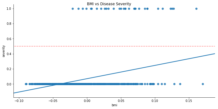
For starters, for our given range of BMI, the best fit line never crosses above 0.5, which means that it will predict for any BMI (within our range) that the disease is non-severe (if we assume anything < 0.5 is non-severe and anything > 0.5 is severe). Also, for lower values of BMI, the line of best fit predicts negative disease progression.

All in all, it does not seem like this is a very good descriptive model when the dependant variable is a categorical variable.

Now let’s look at the same set of data with a logistic regression fit. Logistic regression fits are much the same in theory to linear regression fits, just that instead of fitting a line, we are fitting the logistic function.

If we get mathematical for a moment:

In linear regression we have our equation for a line \(y=mx+c\) where m is the gradient and c the 0-intercept), and we tweak m and c such that the line fits the data the best.
In logistic regression, the equation for the line becomes: \(\frac{1}{1 + e^{-m(x-c)}}\). m and c again control the shape of the graph, but their meanings are less intuitive than gradient and intercept. I won’t get into it here but you can play on WolframAlpha plotting this function for different values of m and c to understand it.

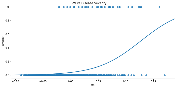
We can see straight away the logistic function provides a much better model of the data:

At extreme values of BMI in our range, the Y-value is above 0.5, hence predicts severe disease progression.
We no longer get negative disease progression predictions.

In general over all sets of categorical data, logistic functions model the situation better, which is why they became the activation function of choice for Neural Networks (to begin with - we now favour other functions like the ReLU which I wll talk about at a later date).

In python, the code would be as follows:

import numpy as np

def sigmoid(z):
    """
    This function implements the logistic function and returns the result. It can operate on vectors.

    :param z: A matrix of dimension (i, m)
        - i is the number of nodes
        - m is the number of training examples

    :return: sigmoid(input)
    """

    return 1 / (1 + np.exp(-z))

Note that in the code above, m is used to mean the number of training examples, not the gradient - this is just a convention thing that I’ve picked up and unfortunately it clashes when we talk about line gradients. In future posts, we will not refer to line gradients anymore so m will solely refer to the number of training examples.

Note that sigmoid is just another name for the logistic function, and here we set m=1 and c=0 so the equation simplifies down.

So with the activation function in place, we have half of our Artifical Neuron already. The other half involves the collection of an arbitrary number of inputs to feed into the activation function.

I will talk about this in the next post! In the meantime, you can find the code I’ve written thus far, all 10 lines of it, at: https://github.com/qichaozhao/potatolemon

-qz

Potatolemon - Logistic Activation Function

Introduction

Logistic Regression

Recent articles