Neuron Weights

Previously, we talked about how the Logistic function is a good basic way to classify a binary outcome (e.g. 0 or 1), and hence makes for a good basic activation function within our artificial model for a neural network.

We know conceptually speaking, that the other half of an artificial neuron has a bunch of weighted inputs that are summed and then fed into the activation function, so if we use a neuron that we model as follows:

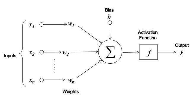
Then, the equation for the output of the neuron will be as follows:

\[y = f(w_{1}x_{1} + w_{2}x_{2} + ... + w_{n}x_{n} + b)\]

In this equation we define the following quantities:

\(y\): the output of the neuron.
\(f()\): the activation function (the logistic function for now)
\(w\): a vector of weights applied to the input (shape of (x, 1))
\(x\): a vector of inputs (shape of (x, 1))
\(b\): a bias value that allows the activation function to be fitted better to the data.

Knowing that these are vectors, we can re-write using matrix multiplication as:

\[y = f(w^{T}.x + b)\]

Extending this a little further - if we wanted to tackle multiple training examples at once, then we can simply stack each element in the equation and turn each of them into a matrix.

This doesn’t change the equation, which becomes (written in capitals as per matrix multiplication convention):

\[Y = f(W^{T}.X + b)\]

But it means the quantities are now:

\(Y\): the output of the neuron for each example, a vector of size (m, 1) where m is the number of examples.
\(f()\): the activation function (the logistic function for now)
\(W\): a matrix of weights applied to the input (shape of (1, x)) where x is the number of input nodes.
\(X\): a matrix of inputs (shape of (x, m)) where m is the number of training examples and x is the number of input nodes.
\(b\): a bias vector that allows the activation function to be fitted better to the data. It has shape (m, 1).

So, after not much math-ing, we have the entire equation that describes the neuron. Now we can go ahead and implement it.

Implementation

We will implement the neuron as a class, so that when we build the network it will be composed of many Neuron objects. Each object can save its own weights, which will hopefully help us when it comes to implementing forward and backpropagation.

"""
The Neuron class.

Holds its own weights and contains getters and setters for it.

Also contains the forward function, used to "activate" the neuron.
"""

import numpy as np

from .activations import sigmoid


class Neuron(object):


    def __init__(self, num_inputs, activation=sigmoid):

        self.activation = activation
        self.num_inputs = num_inputs
        self.weights = np.random.randn(1, num_inputs) * 0.01
        self.bias = 0

    def forward(self, input):
        """
        In this function we implement the equation y = f(W.X + b)

        :param input: a column vector of length (i, m)
            i: num weights, or rather the number of input nodes
            m: num training examples
        :return: a vector of shape (1, m) where m is the number of training examples
        """
        return self.activation(np.dot(self.weights, input) + self.bias)

    def get_weights(self):
        """
        Return the weights

        :return: a weight vector of length num_inputs
        """
        return self.weights

    def set_weights(self, weights):
        """
        Update the weights

        :return:
        """
        self.weights = weights.reshape(1, self.num_inputs)

That’s it for this post.

Next post, things start getting a bit more exciting as we will build some higher level abstractions (Layers and Network) that make it easier to construct a network out of individual neurons.

As with my previous post, all code can be found on the github project: https://github.com/qichaozhao/potatolemon

Peace out for now!

-qz

Potatolemon - Neuron Weights

Previously on Potatolemon…

Neuron Weights

Implementation

Recent articles