Previously on Potatolemon…

Losses

Previously on potatolemon, we finished building out the abstractions for the layer and the network that we’ll rely on in the future to interface with our neural network. This brought us to a point where we have a Multilayer Perceptron (or, a Neural Network that only goes in the forward direction).

Today, we’ll talk about and implement the first part of training a Neural Network - the losses - because the network needs to know how much it is wrong by if it is to begin learning. Losses can also be called costs or errors, and a loss function can also be called a cost function or error function.

To illustrate what we mean by a loss, let’s think back to our logistic regression output from a few blog posts ago. Remember that for a single logistic function, we have a range of outputs between 0 and 1 (you can think of it as a range of probabilities that something might occur, but it’s not quite that).

If we were to use this logistic function in a binary classification problem (i.e. perhaps trying to decide whether a picture is of a cat or not), then we could use our training examples to compare our logistic function output against a ground truth that we already know. In this scenario, a simple way to calculate loss might be to take the difference between the two.

Let’s say for example that if a picture is of a cat, we will give it class label = 1, and if it is not, then we will give it a class label = 0. Then, we run this example through our logistic function. If we get a predicted cat probability of 0.7 but the picture is of a cat (ground truth = 1.0), then our error in this case will be 1.0 - 0.7 = 0.3.

Generalising this, we can define a simple loss function J as follows:

\[J = |y_{true} - y_{pred}|\]

\(y_{true}\) is the label we have assigned (0 or 1)
\(y_{pred}\) is the output of the forward pass (a probability between 0 and 1)

This equation defines the absolute loss (also known as the L1 loss), and is one of many different loss functions that we can apply to measure how well our prediction result matches up against the ground truth.

This L1 loss however is not the best loss metric to use for a classification problem - for that there is something called Cross Entropy. The equation given for the Average Cross Entropy loss is as below:

\[J = - \frac{1}{M} \sum_{m=0}^M \sum_{i=1}^I y_{mi} ln (\hat{y_{mi}}) \qquad (1)\]

\(M\) is the number of training examples.
\(i\) is a class that is being predicted (of a total \(I\) classes)
\(y_{mi}\) is the ground truth of class \(i\) for training example \(n\).
\(\hat{y_{mi}}\) is the predicted value of class \(i\) for training example \(n\).

Although this seems more complicated than for our L1 loss, it is partly because we are firstly summing across all training examples and taking the average, and also because we have to deal with an arbitrary number of classes.

So, why is cross entropy a better loss metric to use L1 loss?

Cross Entropy loss penalises wrong classifications much more harshly than L1 loss.
Cross Entropy loss increases the effectiveness of training a neural network due to how the equation differentiates during backpropagation - it reduces the vanishing gradient problem compared to L1 loss.

For proving point 1, we can take a look at the figure below, which plots the Cross Entropy loss versus L1 loss for varying predictions vs a ground truth of 1.

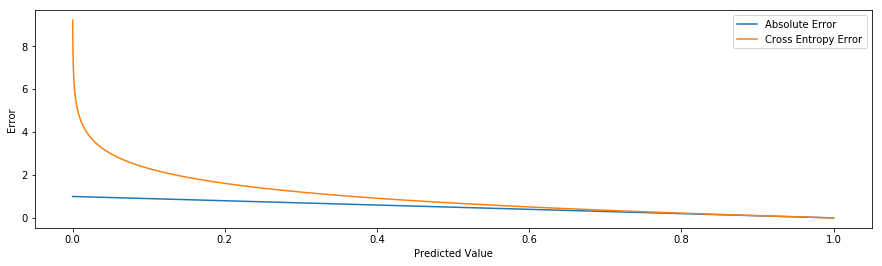
You can see immediately that if our ground truth is 1, we get an exponentially increasing penalty the further away we are if we use log loss (up to an undefined value if we actually predict 0), versus just a linearly increasing penalty (up to a maximum of 1).

For proving point 2 - we will tackle this in a future blog post when we implement the backpropagation algorithm.

So, knowing that we will now choose the Average Cross Entropy, we actually need to end up implementing two variants. One for binary classification and one for multi-class classification.

For a multi class classification, i.e. I > 2, then we end up having one output node per class, which means we can use the Average Cross Entropy loss equation given above.

For a binary classification though, we actually end up just using one output node to represent the two possible outcomes. If the output node is zero then that gives us the first class, and if the output node is one, then that gives us the second class. This results in a slightly different Average Cross Entropy equation that we can derive from the above.

First, we set \(I = 2\) and expand the summation term over all \(i\).

\[J = - \frac{1}{M} \sum_{m=0}^M y_{m1} log (\hat{y_{m1}}) + y_{m2} log (\hat{y_{m2}})\]

Next, we recognise that since we are using one output node to represent two states, the state \(y_{m2}\) can be re-written in terms of \(y_{m1}\). This is because if one state is 1, then the other must be 0.

\[y_{m2} = 1 - y_{m1}\]

Now we can substitute this directly into the equation:

\[J = - \frac{1}{M} \sum_{m=0}^M y_{m1} ln (\hat{y_{m1}}) + (1 - y_{m1}) ln (1 - \hat{y_{m1}}) \qquad (2)\]

And so we get our Average Binary Cross Entropy equation.

Now, all we are left to do is the relatively simple matter of translating our equations (1) and (2) into code.

"""
This file contains all of our cost functions.
"""

import numpy as np


def binary_crossentropy(pred, actual, epsilon=1e-15):
    """
    Calculates the cross entropy loss for a binary classification output (e.g. one output node).

    :param pred: A vector value that is the output from the network of shape (1, m) where m is the number of training examples
    :param actual: A vector value that is the ground truth of shape (1, m) where m is the number of training examples
    :return: A vector value representing the binary_crossentropy loss of shape (1, m) where m is the number of training examples
    """

    # Here we offset zero and one values to avoid infinity when we take logs.
    pred[pred == 0] = epsilon
    pred[pred == 1] = 1 - epsilon

    # m is the number of training examples in this case
    m = pred.shape[1]

    J = -1 / m * np.sum(np.dot(actual, np.log(pred.T)) + np.dot((1 - actual), np.log((1 - pred).T)))
    return J


def categorical_crossentropy(pred, actual, epsilon=1e-15):
    """
    Calculates the average entropy loss for a multi class classification output (e.g. multiple output node).

    :param pred: A vector value that is the output from the network of shape (i, m) where i is the number of classes, and m is the number of training examples
    :param actual: A vector value that is the ground truth of shape (i, m) where i is the number of classes, and m is the number of training examples
    :return: A vector value representing the binary_crossentropy loss of shape (1, m) where i is the number of classes, and m is the number of training examples
    """

    # Here we offset zero and one values to avoid infinity when we take logs.
    pred[pred == 0] = epsilon
    pred[pred == 1] = 1 - epsilon

    i, m = pred.shape

    # We loop through each class and calculate our final cost
    # This could probably be done in a quicker fashion via a matrix multiplication but for simplicity's sake we use a loop
    J = 0
    for cls in range(i):

        pred_cls = pred[cls, :].T
        actual_cls = actual[cls, :]

        J = J + (- 1 / m * np.sum(np.dot(actual_cls, np.log(pred_cls))))

    return J

If you read through the code above, you’ll notice I add in an extra few lines for slightly perturbing prediction values away from absolute 1s and 0s (although these are very unlikely anyway). This must be done to avoid inf values being returned by the np.log function in case our predictions do end up being 1 or 0.

Okay, so that’s all for this post! Slightly more mathsy than we’ve had previously, but I hope it all made sense.

Next post we tackle probably the most interesting part of building a neural network - the backpropagation and weight update. This is what allows the networks to train!

All code can be found on the github project: https://github.com/qichaozhao/potatolemon

Peace out for now!

-qz

Potatolemon - Losses

Previously on Potatolemon…

Losses

Recent articles