Potatolemon - Backpropagation (Part 1)
Searching Google images with the term “backpropagation” is a bit of a cool-image wasteland, so, I hope you enjoy the cute kitten.
Previously on Potatolemon…
Backpropagation (Part 1)
Previously on potatolemon, we built out the loss functions that would be needed when training the network. In this blog post, we’ll tackle the next big part of training a neural network - backpropagation.
A neural network’s predictions are the result of forward propagating an input through the network with its attendant weights and activation functions. Therefore, when we train a network all we’re really doing is adjusting the weights in order to minimise the error.
So, if building out the losses allowed us to see how wrong our network was in its predictions, then backpropagation allows us to propagate the error back through the network in order to assign the correct amount of blame on each neuron so that we can adjust its weights to reduce the loss.
One Neuron
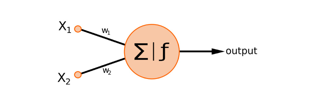
First let’s get an intution for backpropagation before we derive it formally.
If we take the neuron above, which has two input weights and one output, and find an error for it, how might we assign blame?
If the two contributions from the inputs multiplied by the weights to the neuron were equal, then it might make sense to assign blame to the weights in a 50/50 way as well. However, if this is not the case, then we need to assign blame in proportion to the contribution.
Mathematically speaking, we want to calculate a relationship between the change in the loss function and the change in our neuron weights, which means we want to know for this particular neuron the two following things:
\[\frac{\partial J}{\partial w_{1}} \qquad (1)\] \[\frac{\partial J}{\partial w_{2}} \qquad (2)\]Now, we can’t calculate this partial derivative directly, but we can re-write this using the chain rule (just for equation (1) to demonstrate) as follows:
We know from our previous blog post that our loss function (a binary cross entropy loss) is as follows:
\[J = - \frac{1}{N} \sum_{n=0}^N y_{n1} ln (\hat{y_{n1}}) + (1 - y_{n1}) ln (1 - \hat{y_{n1}})\]This relates the loss \(J\) to our prediction output \(\hat{y}\). For simplicities sake, let’s forget about the sum over all training examples \(N\), and write the equation as:
\[J = - (y_{1} ln (\hat{y_{1}}) + (1 - y_{1}) ln (1 - \hat{y_{1}})) \qquad (4)\]In addition to equation (4) above, we also have another equation which links \(\hat{y}\) to the input, and that is:
Where \(\sigma\) is our sigmoid function, so if we expand that then we can write:
\[\hat{y} = \frac{1}{1 + e^{-(W^{T}.X + b)}} \qquad (5)\]With these two equations ((4) and (5)), we can now calculate our two terms in the equation (1). Let’s do the differentiation steps together. First, for \(\frac{\partial J}{\partial \hat{y}}\).
Re-writing the above equation, we get:
\[\frac{\partial J}{\partial \hat{y}} = - \left(\frac{y - \hat{y}}{\hat{y}(1 - \hat{y})} \right) \qquad (6)\]Next, we calculate \(\frac{\partial \hat{y}}{\partial w_{1}}\). To make this easier, we use a substitution:
\[z = W^{T}.X + b = w_{1}x_{1} + w_{2}x_{2} + b\]This means we can re-write the equation as:
\[\frac{\partial \hat{y}}{\partial w_{1}} = \frac {\partial}{\partial w_{1}} \left( \frac{1}{1 + e^{-z}} \right) \frac {\partial z}{\partial w_{1}}\]The sigmoid function differentiates nicely such that \(f'(x) = f(x) (1 - f(x))\), and we know that \(\frac {\partial z}{\partial w_{1}} = x_{1}\) so our equation above becomes:
\[\frac{\partial \hat{y}}{\partial w_{1}} = \sigma(z) (1 - \sigma(z)) x_{1}\]Where \(\sigma(z)\) is our logistic function (writing for readability).
Then, we remember that \(\sigma(z) = \hat{y}\) in this case. Which allows us to make the final substitutions and say that:
\[\frac{\partial \hat{y}}{\partial w_{1}} = \hat{y} (1 - \hat{y}) x_{1} \qquad (7)\]Finally, substituting equations (6) and (7) into equation (3) and simplifying we get the following:
Following the same logic for \(w_{2}\), we get:
\[\frac{\partial J}{\partial w_{2}} = (\hat{y} - y) x_{2}\]And although the bias is not drawn on the figure above, we can (and should) also calculate the backpropgation rule for it. Again following the same logic above, we get:
\[\frac{\partial J}{\partial b} = \hat{y} - y\]These are important results, as they specify our weight updates for the neural network - this is literally how this neuron will train!
Multiple Neurons / Layers
Okay, so, we have derived the backpropagation equation for one of the weights in a situation where there is just one neuron. But how does it look like in the case that the network is more complicated?
Can we come up with a more general formula that can be applied?
The answer is of course yes, and we will work through this in the next post in this series. This means that we are all math and no code in this post, but what are ya gonna do ¯\_(ツ)_/¯
See you in the next post!
-qz