This week, we continue with the cute but irrelevant title picture theme!

Previously on Potatolemon…

Backpropagation (Part 2)

Previously on potatolemon, we derived the mathematics for how to update weights via backpropagation for one Neuron. We saw how it was possible via the chain rule to recursively work backwards through the neuron to arrive at our weight update equations.

In this post, we’ll extend on what was done previously and derive the equations again for an arbitrary neuron in an arbitrary network, which gives us a general equation that we can then implement in code.

One Arbitrary Neuron

Let’s start with a diagram of an arbitrary neuron somewhere in our fully connected network. It looks like the following:

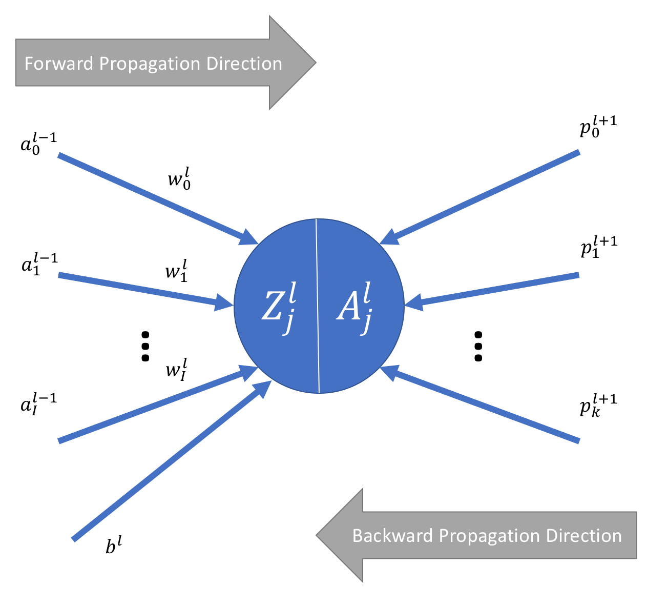
Starting from left to right, the quantities we are dealing with are as follows:

\(a_{i}^{l-1}\) - indicates the activation output \(a\) from the neuron \(i\) in layer \(l-1\).
\(w_{i}^{l}\) - indicates the weight \(w\) for the connection between neuron \(i\) in layer \(l-1\) and the current neuron in layer \(l\).
\(b^{l}\) - indicates the bias input for layer \(l\).
\(Z_{j}^{l}\) - indicates the output of the equation \(W.X + b\) for this neuron.
\(A_{j}^{l}\) - indicates the activation output for this neuron.
\(p_{k}^{l+1}\) - indicates the backpropagation output (i.e. the input travelling in the backwards direction) from the neuron \(k\) in layer \(l + 1\).

Now we’ve defined the quantities that are involved, let’s remind ourselves of the equations we are trying to derive, namely weight updates for each of the parameters (\(W\) and \(b\)), that is:

\[\frac{\partial J}{\partial W^{l}} \qquad (1)\] \[\frac{\partial J}{\partial b^{l}} \qquad (2)\]

Note for the capitalised weight \(W\) we define it to be a vector of weights for this neuron thus we no longer write the subscript.

We can re-write these equations using the chain rule. For equation (1) this becomes:

\[\frac{\partial J}{\partial W^{l}} = \frac{1}{M} \left( \frac{\partial J}{\partial Z^{l}} . (A^{l-1})^{T} \right) \qquad (3)\]

Note \(M\) in this case indicates the number of training examples we have. This has been added for completeness-sake. When going through the derivations for the first time you can set M = 1 and treat it as if taking one input at a time.

Using the chain rule again, we can re-write \(\frac{\partial J}{\partial Z^{l}}\) as:

\[\frac{\partial J}{\partial Z^{l}} = \sigma(Z_{j}^{l})(1 - \sigma(Z_{j}^{l})) . \frac{\partial J}{\partial P^{l+1}} \qquad (4)\]

How does this help? Well, we realise that the first part of this equation is purely dependent on our input, and the second part comes from the backpropagation input into the neuron, and can be written as:

\[\frac{\partial J}{\partial P^{l+1}} = \sum_{k=0}^{K} p_{k}^{l+1} \qquad (5)\]

Substituting equation (5) into (4) and then the result into equation (3), we can now write an equation for (1) in terms of known quantities, and that covers our weight updates!

We won’t write the full equation out, because when we come to code it, we will (for the purposes of readability) calculate equation (4) first, then use that in equation (3). Note we don’t actually need to calculate equation (5), since it is the backpropagation input into the neuron, we will have that to hand.

We follow a similar logic for deriving the bias update, to achieve the bias update equation:

\[\frac{\partial J}{\partial b^{l}} = \frac{1}{M} \sum_{m=0}^{M} \frac{\partial J}{\partial Z^{l(t)}} \qquad (6)\]

With these equations, we can now perform the update operations for our neuron parameters, but, we must make sure that backpropagation can continue past this neuron as well, thus we must make one final calculation which will provide the \(l-1\) th layer with the requisite input necessary for them to do backpropagation. This quantity is:

\[\frac{\partial J}{\partial P^{l}} = \frac{\partial J}{\partial A^{l-1}} = (W^{l})^{T} . \frac{\partial J}{\partial Z^{l}} \qquad (7)\]

Luckily, this is quite easy as we already have the equation for \(\frac{\partial J}{\partial Z^{l}}\), it is equation (4) which we derived earlier!

Weight Updates

After backpropagation is finished, we have for each Neuron two main things dw and db - these are the weight and bias updates respectively.

We simply update the existing weights and biases by subtracting the dw and db quantities. This is Stochastic Gradient descent.

Implementation

Right - now that we have got the maths done, we can go ahead and do the implementation.

I don’t necessarily want to make this part of the post a wall of code, as there are a number of changes that were made throughout the various parts of the program, so I will just summarise the changes below:

Any function that was used during forward propagation now has a backward component that calculates the backward propagation component. This is essentially every single component of the library.
A new function under the module optimisers was introduced in order to perform the weight/bias updates (via Stochastic Gradient Descent).
The high level interface on the network (fit) was completed.

Finally a lot of new unit tests were written to test the backwards steps and the code was tested to pass these.

And, that leaves us with a completed Neural Network library than we can in theory start training on tasks!

Validation on XOR

In order to test drive our completed library, we can give it a small toy problem to learn. The XOR problem (learning the output of an XOR gate) is a good one to start with as its a non-linear problem that’s easy to represent analytically and also easy to learn with a multi-layer network.

For the XOR gate, we have the truth table as below:

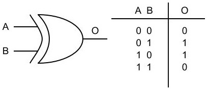
So, we need to output 1 if A or B is 1, but 0 otherwise.

First, let’s tackle this problem using a proper neural network library - pyTorch. We build a very simple architecture which should be able to solve the problem without issue.

Another small detail here is that instead of using sigmoid activations for the hidden layers, we switch to using tanh activations (which are very similar). This is because for some reason when I tried to test it using sigmoid activations the network didn’t learn! If you can explain why I would love to hear from you!

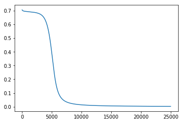
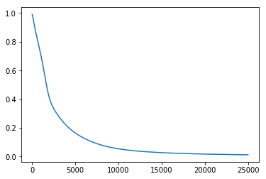
After training for 25,000 epochs on the above truth table (which takes a snappy 4.77 seconds), the losses looked like this:

After training, the network was able to make the following predictions for the output of the truth table:

tensor([[ 0.0023],
        [ 0.9952],
        [ 0.9986],
        [ 0.0025]])

If you recall that our actual truth table is 0, 1, 1, 0, this means the network has pretty much successfully learned the XOR function, it will be able to predict with 100% accuracy the outcomes.

Next, we try using our potatolemon network implementing the exact same architecture, and training for 25,000 epochs also (which took a respectable 6.3 seconds). We get the following costs:

After training, the network was able to make the following predictions:

[[ 0.00324411]
 [ 0.99917027]
 [ 0.99924255]
 [ 0.02033314]]

This looks very close to the pyTorch results, which suggests that our implementation is working as expected! Excitingness!

Although this is very positive news, through testing I have noticed that my library seems very susceptible to initial conditions (e.g. using different numpy random seeds, or even re-running can produce different results that cause the training to not converge). This probably points to a flaw somewhere within the implementation that needs to be addressed using a finer combed testing technique like gradient checking.

However, having said that, neural networks in general can be very susceptible to initalialisation and it can make the difference between learning and not learning. This is especially true when the network is small, as it then becomes more likely to fall into local minima.

In the next post, we’ll continue to explore the performance characteristics of this library.

The code for the tests above can be found at: https://github.com/qichaozhao/potatolemon/blob/master/examples/xor_validation.ipynb

All the rest of the code can be found on the github project: https://github.com/qichaozhao/potatolemon

Peace out for now!

-qz

Potatolemon - Backpropagation (Part 2)