Speeding up Python
This week at work, I hit a performance brick wall with python, which therefore gave me an excuse to dive into the interesting world of code optimisation.
In this post I’ll cover the approaches I used, and give a brief introduction to each of the following:
- Cython
- Numba
- Parallel Processing
- Vectorisation
Excited yet? Yes? Good. Read on!
The problem I faced was to find a way to speed up a row-wise calculation on a large pandas DataFrame. In the first iteration of the code, the calculation was taking so long that it was not scalable to the degree required. Not being one to back down from a challenge, I set about to see what I could do to give the script a proverbial kick up the backside, and maybe at the same time hook it up to some NOS.
For the purposes of this post, I will use an example that involves the following toy dataset. Because, y’know, the actual code is a bit long and complicated (and may also be mildly proprietary).
# Import pandas and numpy, and create our test dataframe (100k rows, random normal)
import pandas as pd
import numpy as np

df = pd.DataFrame(np.random.randn(100000, 2), columns=['A','B'])
This is just a dataframe that’s 100,000 rows long, filled with random numbers.
Let’s say I then want to apply some kind of row-wise function to this dataset, which we can define for the purposes of demonstration as:
# The naive implementation of our calculation function.
def intensive_calculation(row):
    x = row['A'] + row['B']
    return x * (row['A'] * row['A'] / row['B'] * row['B'])
Let’s run this naive implementation using Jupyter Notebook’s magic %%timeit function, which lets us know how long a notebook cell took to execute.
%%timeit
# Running our naive implementation and measuring the time.
df['C'] = df.apply(intensive_calculation, axis=1)
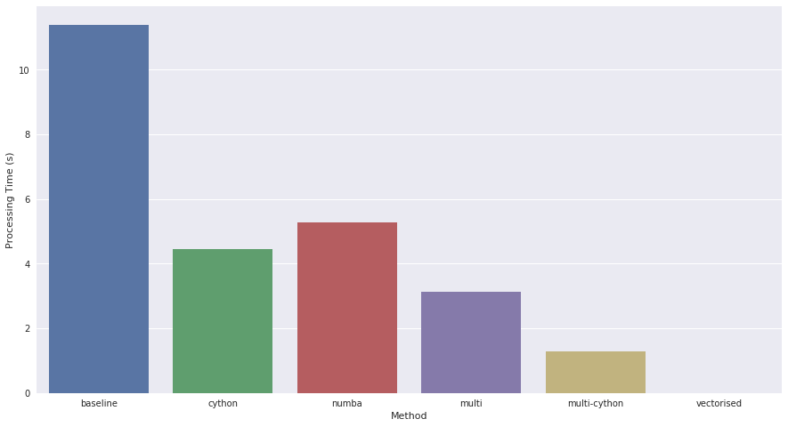
1 loop, best of 3: 11.4 s per loop
So, now we have a baseline, where do we go from here?
Well, from my own experiences, I feel that optimising code generally falls into 3 categories, which I’m going to list in order of potential gains.
- Code Design - The first thing to consider is always the design of the code. A few example things to think about are:
- Unnecessary code - whichever code is being repeated should be pared back to contain only the minimum possible number of commands. The rest should be moved to be outside of the loop.
- Vectorisation - if we can re-write our code to be a vector operation rather than a loop, it’ll usually run a whole lot faster. Mainly because pandas has very efficient vectorised implementations.
- Memoisation - can we make use of a cache to avoid having to re-calculate values?
-
Parallelisation
- Using Cython / Numba to pre-compile or just-in-time compile code.
We’re going to cover them in reverse order. :)
Using Cython / Numba
One of the features of Python that gives it a reputation as a “slow” language is that it is interpreted.
What this means (at a high level) is that each line of code is executed directly, contrast this with a compiled language (such as C / C++) which before execution will translate the written code into machine language specific to the processor that is going to execute the code, allowing optimisations to take place.
To be completely technically accurate, interpreted languages also being end up translated into machine language (through the interpreter), but because the interpreter translates each line of code independently, it is unable to utilise code optimisations that would otherwise be possible.
Python also does not help things by being a dynamically typed language, which means that a variable type can change depending on the value being assigned to it. This entails quite a large processing overhead compared to static typing (where the type is immutable unless explicitly cast to a different type).
Cython and Numba attempt to solve these problems in similar but different ways:
- Cython allows us to write python code which will be compiled into C code before execution. This will run faster than “pure python” code.
- Numba essentially does the same thing, except instead of pre-compiling into C, it uses the LLVM compiler to compile as and when it is needed. The documentation specifically mentions that it is optimised to deal with arrays, so it may not be the perfect fit for our example here, but I will include it just to show how it’s done.
Cython
Great, now that we know all that, let’s see what we can do. First up, Cython. Let’s re-write our function using Cython.
# The Cython implementation of our calculation function.
cpdef double intensive_calc_cython(double a, double b) except *:
    cdef double x

    x = a + b
    return x * (a * a / b * b)
Here is what’s different to our standard python implementation:
defbecomescpdef. Note we also add the lineexcept *to the end of our function declaration. This allows the Cython code to surface exceptions back to the calling function.- We declare variable types for the following variables:
- The function arguments (
double a,double b). - The function return (
double intensive_calc_cython()) - Any internal variables we use in the function (
cdef double d)
- The function arguments (
We can save this into a separate file (I called mine helper.pyx), and use it in our main code as follows:
%%timeit
# Running our Cython implementation
import pyximport
pyximport.install()

from helper import intensive_calc_cython

df['C'] = df.apply(lambda row: intensive_calc_cython(row['A'], row['B']), axis=1)
1 loop, best of 3: 4.46 s per loop
It essentially just becomes a python module we can import and use, except, it’s faster! Note that in order also to use Cython I am no longer passing the pandas series object for the row to the function, but instead the separate values for Column A and B. Cython does not support the pandas series data type so we have to pass more primitive types to it.
Running the code shows that we’ve decreased runtime by ~2.6x. Not bad for something that is pretty simple!
If you are just using Jupyter Notebooks, there’s not even any need to create a separate file, by using the %%cython magic command, you can write Cython directly in a cell.
%load_ext cython
%%cython
# Inline Cython implementation
cpdef double intensive_calc_cython(double a, double b) except *:
    cdef double x

    x = a + b

    return x * (a * a / b * b)
Numba
To make Numba work, it is even easier than Cython! We can just add a decorator onto our function. Note we are again declaring in the decorator the output and input data types. The other parameters I leave you to explore in the Numba documentation!
# using Numba
from numba import jit, float32

# The Numba implementation of our calculation function.
@jit(float32(float32, float32), nopython=True, cache=True)
def intensive_calculation(a, b):
    x = a + b
    return x * (a * a / b * b)
Running this for our test, we get the following: 1 loop: 5.29s per loop. This backs out to an improvement of ~2.2x, not quite as good as Cython (we are not doing any work with arrays after all), but fairly comparable.
Parallel Processing
I have 4 cores on my CPU. Python by and large is single threaded and single processed, which means when running calculations on large dataframes, only one CPU core is being used. Seems like a waste, no?
For our specific case of speeding up row-wise calculations on a dataframe, we can easily split the dataframe up into chunks to parallelize, but in general, application of this technique will need to be well considered as parallelisation means that things will not necessarily execute in the order that it is written, and can in the worst cases lead to deadlocks and race conditions.
For this example though, we are in a prime position to go ahead and employ it.
# Running our naive implementation with multiprocessing
from multiprocessing import Pool
from multiprocessing import cpu_count

def parallelize(df, func):
    """
    This function splits our dataframe and performs the passed function on each split, then combines.
    """

    num_cores = cpu_count()

    df_splits = np.array_split(df, num_cores)
    pool = Pool(num_cores)

    out_df = pd.concat(pool.map(func, df_splits))

    pool.close()
    pool.join()

    return out_df


def intensive_calc_wrapper(df):
    """
    This is the actual function that is being applied.
    """
    return df.apply(lambda row: intensive_calculation(row), axis=1)

df['C'] = parallelize(df, intensive_calc_wrapper)
1 loop: 3.13s per loop.
The parallelize function creates a pool of workers (using the Pool class), that is equal to the number of CPU cores that it has detected. We then split up the dataframe into this number of chunks (4 in my case), and the pool.map function will iterate through our list of inputs (which are the chunks of our dataframe), and apply the function func to each input, assigning the job to the next free worker.
func in this case is the function we define below as intensive_calc_wrapper, which applies our original intensive_calculation function onto whatever dataframe is passed into it.
We can see that parallelisation works pretty well! Giving us an increase of ~3.6x.
We can improve things even further by stacking our parallel code with our Cython function (but this doesn’t work with Numba due to the just-in-time compilation scheme that is used). The code to do this is:
# Running our Cython implementation with multiprocessing
import pyximport
pyximport.install()

from helper import intensive_calc_cython

from multiprocessing import Pool
from multiprocessing import cpu_count

def parallelize(df, func):
    """
    This function splits our dataframe and performs the passed function on each split, then combines.
    """

    num_cores = cpu_count()

    df_splits = np.array_split(df, num_cores)
    pool = Pool(num_cores)

    out_df = pd.concat(pool.map(func, df_splits))

    pool.close()
    pool.join()

    return out_df


def intensive_calc_wrapper(df):
    """
    This is the actual function that is being applied.
    """
    return df.apply(lambda row: intensive_calc_cython(row['A'], row['B']), axis=1)

df['C'] = parallelize(df, intensive_calc_wrapper)
1 loop: 1.28s per loop.
This yields a cool ~8.9x speed improvement.
So, is this best we can do? With Cython and Parallelisation, yes. But we have one more thing to look at, which is our code design.
Vectorisation
For this example, it’s fairly obvious to see that there exists a simple vectorised solution. So let’s implement that and see how we do:
%%timeit
# The fully vectorized time
df['C'] = (df['A'] + df['B']) * (df['A'] * df['A'] / df['B'] * df['B'])
100 loops, best of 3: 4.82 ms per loop
This is ~2365x quicker than our baseline, and ~265x quicker than the best we were able to do with Cython & Parallelisation. That’s not a typo. It’s also worth noting that for this operation, we could even apply multi-processing (since this was done on just 1 core) to potentially speed things up even more!
Conclusions
I think the results speak for themselves.
It is definitely not that difficult to make use of libraries like Numba and Cython to speed up Python code. In particular cases, multiprocessing is not that difficult either. However, there is still no shortcut to fully analysing and writing well designed code to begin with. In this particular example (and indeed I believe for most row-wise dataframe processing tasks), vectorisation is the silver bullet that if successfully implemented, can allow Python to run very fast indeed.
Using the same techniques above, I was able to realise a speed increase of ~6x on my tricky work project challenge. Unfortunately, I was not able to find a vectorised implementation. However fortunately, this effort, along with SQL optimisations made to the data ingestion portion of the pipeline yielded enough improvement such that I was able to achieve the scaleability targets we needed for the project to go ahead.
Bonza! Job done!
For full code and notebooks, see the repository here.
-qz